The Numerical Discretization
Consider the following discretization,
with \(N_x\) intervals, thus having \(\Delta r_i = \frac{R_i}{N_x}\)
and timestep \(\Delta t\).
Let’s define the approximations:
\[\begin{split}\tilde{s}_{b}^{n} &= S_b(n \Delta t) \\
\tilde{s}_{j,i}^{n} &= S(n \Delta t, j \Delta r_i, R_i)\end{split}\]
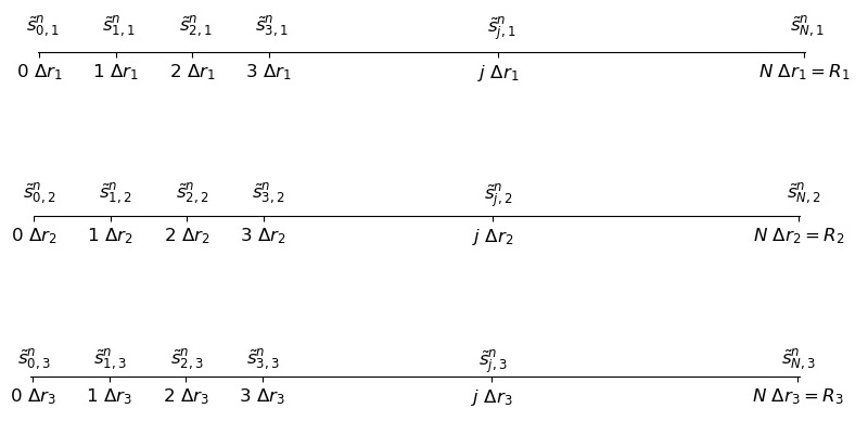
Consider the figure:
For each timestep \(\Delta t\), we have \(N_x+1\) unknowns in each particle size, and one
unknown in the bulk phase, so the total number of unknown are \((N_x+1) N_R + 1\).
The time partial derivative can be discretized as:
\[\frac{\partial S}{\partial t} (n \Delta t, j \Delta r_i, R_i)
\approx
\frac{\tilde{s}^{n+1}_{j,i} - \tilde{s}^{n}_{j,i}}{\Delta t}\]
The central implicit discretization for the first and second partial space derivatives are:
\[\begin{split}\frac{\partial S}{\partial r}(n\Delta t, j \Delta r_i, R_i)
& \approx
\frac{1}{2} \frac{\tilde{s}^{n+1}_{j+1,i}-\tilde{s}^{n+1}_{j-1,i}}{2 \Delta r_i}
+ \frac{1}{2} \frac{\tilde{s}^{n}_{j+1,i}-\tilde{s}^{n}_{j-1,i}}{2 \Delta r_i} \\
\frac{\partial^2 S}{\partial r^2}(n\Delta t, j \Delta r_i, R_i)
& \approx
\frac{1}{2} \frac{\tilde{s}^{n+1}_{j+1,i} -2 \ \tilde{s}^{n+1}_{j,i} + \tilde{s}^{n+1}_{j-1,i}}{(\Delta r_i)^2}
+
\frac{1}{2}\frac{\tilde{s}^{n}_{j+1,i} -2 \ \tilde{s}^{n}_{j,i} + \tilde{s}^{n}_{j-1,i}}{(\Delta r_i)^2}\end{split}\]
The one-sided discretization for the first space derivatives are:
\[\begin{split}\frac{\partial S}{\partial r}(n \Delta t,0, R_i)
& \approx \frac{ - 3 \ \tilde{s}^{n}_{0,i} + 4 \ \tilde{s}^n_{1,i} - \tilde{s}^{n}_{2,i}}{2 \Delta r} \\
\frac{\partial S}{\partial r}(n \Delta t,N_x \Delta r_i, R_i)
& \approx \frac{ \tilde{s}^{n}_{N_x-2,i} - 4 \ \tilde{s}^n_{N_x-1,i} + 3\tilde{s}^{n}_{N_x,i}}{2 \Delta r}\end{split}\]
The reaction-diffusion equation is:
\[\begin{split}\tilde{s}^{n+1}_{j} - \frac{\Delta t D_S}{2 (\Delta r)^2} \left[ \left( 1-\frac{2}{j} \right) \tilde{s}^{n+1}_{j-1} -2 \ \tilde{s}^{n+1}_{j} + \left(1+\frac{2}{j} \right)\tilde{s}^{n+1}_{j+1} \right] \\
= \\
\tilde{s}^{n}_{j} + \frac{\Delta t D_S}{2 (\Delta r)^2} \left[ \left(1-\frac{2}{j}\right)\tilde{s}^{n}_{j-1} -2 \ \tilde{s}^{n}_{j} + \left( 1+\frac{2}{j} \right) \tilde{s}^{n}_{j+1} \right] \\
- \Delta t \ v_e (\tilde{s}^{n+1}_{j,i}) \ I(n \Delta t) \ Z( j \Delta r_i, R_i)\end{split}\]
The boundary condition at \(r=0\) gets discretized as
\[-3 \tilde{s}^{n+1}_0 + 2 \tilde{s}^{n+1}_1 + \tilde{s}^{n+1}_2 = 0\]
The continuity conditions at \(r=R_i\) are:
\[\begin{split}\tilde{s}^{n}_{b} & = \tilde{s}^{n}_{N_x, i} \textrm{ for } i \in \{ 1, 2, \cdots, N_R \} \\
\tilde{s}^{n+1}_{b} + \sum_{i=1}^{N_c} \gamma_i (\tilde{s}^{n+1}_{N_x-2, i} + 2 \ \tilde{s}^{n+1}_{N_x-1, i} - 3 \ \tilde{s}^{n+1}_{N_x, i})
&= \tilde{s}^{n}_{b} - \sum_{i=1}^{N_c} \gamma_i (\tilde{s}^{n}_{N_x-2, i} + 2 \ \tilde{s}^{n}_{N_x-1, i} - 3 \ \tilde{s}^{n}_{N_x, i})\end{split}\]
where \(\gamma_i=\frac{3 D_s V_c}{V_R E[R^3]} N_x^2 \Delta r_i\)
The initial condition at the surface of the particles are
\[\begin{split}\tilde{s}_b(0) &= S_0 \\
\tilde{s}_{j,i}^{0} &= 0 \textrm{ for } 0 \leq j < N_x\end{split}\]
The Numerical Implementation
We stack the vectors and explicitely replace \(\tilde{s}^{n}_{b} = \tilde{s}^{n}_{N_x, i}\),
so the vector has size \(Nx N_R +1\). We will use the notation \(s^{n}_{j + i N_x} = \tilde{s}^{n}_{j,i}\)
and \(s^{n}_{N_x N_R + 1} = s^{n}_{b}\).
For each time step, we must solve:
\[(I + A) \vec{s}^{n+1} = (I - A) \vec{s}^{n} + \Delta t \vec{v}^n\]
As the matrices are fixed (do not depend on the time variable), they can be computed and stored.
A PLU factorization (Permutation Lower Upper) is computed for efficiently solve the equation in each time step.
The vectors and matrices are defined as:
\[\begin{split}\vec{s}^{n} =
\left( \begin{array}{c}
s^{n}_{0} \\
s^{n}_{1} \\
s^{n}_{2} \\
\vdots \\
s^{n}_{N_x-3} \\
s^{n}_{N_x-2} \\
s^{n}_{N_x-1} \\ \hline
\vdots \\ \hline
s^{n}_{(N_c-1) N_x} \\
s^{n}_{(N_c-1) N_x + 1} \\
s^{n}_{(N_c-1) N_x + 2} \\
\vdots \\
s^{n}_{(N_c-1) N_x + N_x-3} \\
s^{n}_{(N_c-1) N_x + N_x-2} \\
s^{n}_{(N_c-1) N_x + N_x-1} \\ \hline
s^{n}_{N_R N_x+1}
\end{array} \right)
=
\left( \begin{array}{c}
s^{n}_{0,1} \\
s^{n}_{1,1} \\
s^{n}_{2,1} \\
\vdots \\
s^{n}_{N_x-3,1} \\
s^{n}_{N_x-2,1} \\
s^{n}_{N_x-1,1} \\ \hline
\vdots \\ \hline
s^{n}_{0,N_c} \\
s^{n}_{1,N_c} \\
s^{n}_{2,N_c} \\
\vdots \\
s^{n}_{N_x-3,N_c} \\
s^{n}_{N_x-2,N_c} \\
s^{n}_{N_x-1,N_c} \\ \hline
s^{n}_{b}
\end{array} \right)\end{split}\]
\[\begin{split}I = \left[ \begin{array}{ccccccc|c|ccccccc|c}
0 & & & & & & & \cdots & & & & & & & & \\
& 1 & & & & & & \cdots & & & & & & & & \\
& & 1 & & & & & \cdots & & & & & & & & \\
& & & \ddots & & & & \cdots & & & & & & & & \\
& & & & 1 & & & \cdots & & & & & & & & \\
& & & & & 1 & & \cdots & & & & & & & & \\
& & & & & & 1 & \cdots & & & & & & & & \\ \hline
\vdots & \vdots & \vdots & \vdots & \vdots & \vdots & \vdots & \ddots & \vdots & \vdots & \vdots & \vdots & \vdots & \vdots & \vdots & \\\hline
& & & & & & & \cdots & 0 & & & & & & & \\
& & & & & & & \cdots & & 1 & & & & & & \\
& & & & & & & \cdots & & & 1 & & & & & \\
& & & & & & & \cdots & & & & \ddots & & & & \\
& & & & & & & \cdots & & & & & 1 & & & \\
& & & & & & & \cdots & & & & & & 1 & & \\
& & & & & & & \ddots & & & & & & & 1 & \\ \hline
& & & & & & & \ddots & & & & & & & & 1 \\
\end{array} \right]\end{split}\]
\[\begin{split}A = \left[ \begin{array}{ccccccc|c|ccccccc|c}
-3 & 2 & 1 & & & & & \cdots & & & & & & & & \\
a_{2,1} & b_{2,1} & c_{2,1} & & & & & \cdots & & & & & & & & \\
& a_{3,1} & b_{3,1} & c_{3,1} & & & & \cdots & & & & & & & & \\
& & & \ddots & & & & \cdots & & & & & & & & \\
& & & a_{N_x-3,1} & b_{N_x-3,1} & c_{N_x-3,1} & & \cdots & & & & & & & & \\
& & & & a_{N_x-2,1} & b_{N_x-2,1} & c_{N_x-2,1} & \cdots & & & & & & & & \\
& & & & & a_{N_x-1,1} & b_{N_x-1,1} & \cdots & & & & & & & & c_{N_x-1,1} \\ \hline
\vdots & \vdots & \vdots & \vdots & \vdots & \vdots & \vdots & \ddots & \vdots & \vdots & \vdots & \vdots & \vdots & \vdots & \vdots & \\\hline
& & & & & & & \cdots & -3 & 2 & 1 & & & & & \\
& & & & & & & \cdots & a_{2,N_R} & b_{2,N_R} & c_{2,N_R} & & & & & \\
& & & & & & & \cdots & & a_{3,N_R} & b_{3,N_R} & c_{3,N_R} & & & & \\
& & & & & & & \cdots & & & & \ddots & & & & \\
& & & & & & & \cdots & & & & a_{N_x-3,N_R} & b_{N_x-3,N_R} & c_{N_x-3,N_R} & & \\
& & & & & & & \cdots & & & & & a_{N_x-2,N_R} & b_{N_x-2,N_R} & c_{N_x-2,N_R} & \\
& & & & & & & \cdots & & & & & & a_{N_x-1,N_R} & b_{N_x-1,N_R} & c_{N_x-1,N_R}\\ \hline
& & & & & -\gamma_1 & -2 \gamma_1 & \cdots & & & & & & -\gamma_1 & -2 \gamma_{N_R} & 3 \sum_{i=1}^{N_R} \gamma_i \\
\end{array} \right]\end{split}\]
\[\begin{split}\vec{v}^{n} =
\left( \begin{array}{c}
0 \\
V(s^{n}_{1,1}) \ I(n \Delta t) \ Z(1 \Delta r_1, R_1)\\
V(s^{n}_{2,1}) \ I(n \Delta t) \ Z(2 \Delta r_1, R_1)\\
\vdots \\
V(s^{n}_{N_x-3,1}) \ I(n \Delta t) \ Z( (N-x-3) \Delta r_1, R_1)\\
V(s^{n}_{N_x-2,1}) \ I(n \Delta t) \ Z( (N-x-2) \Delta r_1, R_1)\\
V(s^{n}_{N_x-1,1}) \ I(n \Delta t) \ Z( (N-x-1) \Delta r_1, R_1)\\ \hline
\vdots \\ \hline
0 \\
V(s^{n}_{1,N_c}) \ I(n \Delta t) \ Z(1 \Delta r_{N_c}, R_{N_c})\\
V(s^{n}_{2,N_c}) \ I(n \Delta t) \ Z(2 \Delta r_{N_c}, R_{N_c})\\
\vdots \\
V(s^{n}_{N_x-3,N_c} \ I(n \Delta t) \ Z( (N_x-3) \Delta r_{N_c}, R_{N_c})\\
V(s^{n}_{N_x-2,N_c} \ I(n \Delta t) \ Z( (N_x-2) \Delta r_{N_c}, R_{N_c})\\
V(s^{n}_{N_x-1,N_c} \ I(n \Delta t) \ Z( (N_x-1) \Delta r_{N_c}, R_{N_c})\\ \hline
0
\end{array} \right)\end{split}\]